Contents
Estimating Continuous-time Transfer Function Models in Closed Loop
This example illustrates how you can use the CONTSID toolbox tools to determine a continuous-time transfer function model in closed loop. We begin by simulating experimental data and use the Closed-Loop version of the Simple Refined Instrumental Variable (CLSRIVC) estimation method to estimate continuous-time models from the data. The following estimation routine is illustrated in this example: clsrivc.
close all
Closed-loop System Description
This demo considers a system in closed-loop as repressented below
                     +------+   |r    +------+         | e
                     |      |   |  u  |      |    x    |
         0 --->O---->   C   |---+--->    G   |---------+---> y
               |     |      |         |      |         |
              -|     +------+         +------+         |
               |                                       |
               +---------------------------------------+
The process is denoted by G and the controller by C which is assumed to be known here. An external excitation signal r is added to the controller output. The identification problem is to find estimates of the process G from measured data sequences of r, u and y of respectively, the external signal, the process input and output.
Generating the Data for Analysis
Consider a continuous-time SISO second-order system without delay described by the following transfer function:
            s + 1
G(s) =  ---------------
         s^2 + 0.5s + 1
where s denotes the differentiation operator. Create first an IDPOLY model structure object describing the true continuous-time plant model. ...,'Ts',0) indicates that the system is time-continuous.
  N0=[0 1 1];
  D0=[1 0.5 1];
  M0=idpoly(1,N0,1,1,D0,'Ts',0)
M0 =
Continuous-time OE model:  y(t) = [B(s)/F(s)]u(t) + e(t)
  B(s) = s + 1

  F(s) = s^2 + 0.5 s + 1

Parameterization:
   Polynomial orders:   nb=3   nf=2   nk=0
   Number of free coefficients: 5
   Use "polydata", "getpvec", "getcov" for parameters and their uncertainties.

Status:
Created by direct construction or transformation. Not estimated.
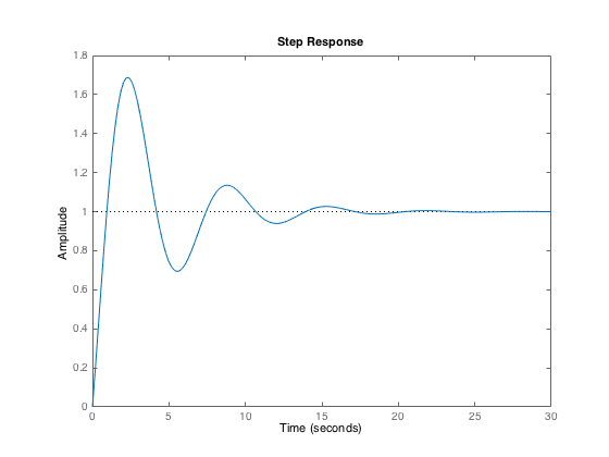
Plot the step response from which it can be observed that the system response is quite underdamped
step(M0)
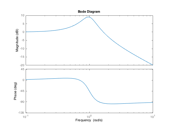
Plot now the frequency response from which it can be seen that the mode of the system is around 1 rad/sec.
bode(M0);
A first-order controller is used and is described by the following transfer function model:
          10s + 15
C(s) =  ---------------
             s
Define transfer function model describing the controller. The polynomials are entered in descending powers of s.
  Nc=[10 15];
  Dc=[1 0];
  Mc=tf(Dc/Dc(1),Nc/Dc(1));
We then compute the closed-loop tranfer functions along with the IDPOLY model structure objects.
  Bcl = conv(N0,Dc);
  Acl = conv(D0,Dc)+conv(N0,Nc);
  Ccl = conv(D0,Dc);
  Dcl = conv(D0,Nc);

  Ecl = conv(N0,Nc);

  M0yr=idpoly(1,Bcl,1,1,Acl,'Ts',0);
  M0ur=idpoly(1,Ccl,1,1,Acl,'Ts',0);
  M0ud=idpoly(1,Dcl,1,1,Acl,'Ts',0);
We take a PRBS of maximum length with 7500 points as external signal r. r is added on the controller output signal. The sampling period is chosen to be 0.005s.
  r = [0;prbs(4,500)];
  Ts= 0.005;
We then create a DATA object for the input external signal with no output the input r and sampling interval Ts. The input intersample behaviour is specified by setting the property 'Intersample' to 'zoh' since the input is piecewise constant here.
datar = iddata([],r,Ts,'InterSample','zoh');
The noise-free process input and output are simulated with the SIMC routine and stored in udet and ydet.
  udet = simc(M0ur,datar);
  ydet = simc(M0yr,datar);
We then create 2 noise-free data objects to be used in the following: - datadet_yr with output ydet, input r and sampling interval Ts; - datadet_yu with output ydet, input udet and sampling interval Ts.
  datadet_yr = iddata(ydet,r,Ts,'InterSample','zoh');
  datadet_yu = iddata(ydet,udet,Ts,'InterSample','zoh');
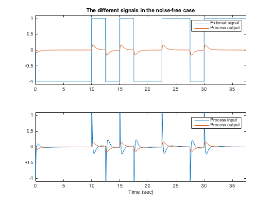
Let us have a look to the different noise-free signals involved.
  N=length(r);
  t=[0:Ts:(N-1)*Ts];
  subplot(2,1,1)
  plot(t,r,t,ydet),legend('External signal','Process output')
  axis([0 t(end) -1.1 1.1])
  title('The different signals in the noise-free case')
  subplot(2,1,2)
  plot(t,udet,t,ydet),legend('Process input','Process output')
  axis([0 t(end) -1.1 1.1])
  xlabel('Time (sec)')
Closed-loop Identification in the Noise-free Situation
We first identify a continuous-time model in the noise-free case by using the Closed-Loop version of the Simple Refined Instrumental Variable CLSRIVC function. The extra information required are: - the IDDATA object datadet_yu with process output ydet, input udet - the IDDATA object datadet_yr with output ydet, external signal r - the number of numerator and denominator parameters to be estimated and the number of samples for the delay: [nb nf nk]=[2 2 0]; - the controller IDPOLY model. The CLSRIVC function can now be used as follows:
Mclsrivc=clsrivc(datadet_yu,datadet_yr,[2 2 0],Mc)
Mclsrivc =
Continuous-time OE model:  y(t) = [B(s)/F(s)]u(t)
  B(s) = 0.9755 s + 0.9755

  F(s) = s^2 + 0.5492 s + 1.012

Parameterization:
   Polynomial orders:   nb=2   nf=2   nk=0
   Number of free coefficients: 4
   Use "polydata", "getpvec", "getcov" for parameters and their uncertainties.

Status:
Estimated using Contsid CLSRIVC method on time domain data.
Fit to estimation data: 100.00
FPE: 2.986e-31, MSE 2.982e-31
Let us compare the identified model with the true process model. As seen below, they are very close
M0,
M0 =
Continuous-time OE model:  y(t) = [B(s)/F(s)]u(t) + e(t)
  B(s) = s + 1

  F(s) = s^2 + 0.5 s + 1

Parameterization:
   Polynomial orders:   nb=3   nf=2   nk=0
   Number of free coefficients: 5
   Use "polydata", "getpvec", "getcov" for parameters and their uncertainties.

Status:
Created by direct construction or transformation. Not estimated.
Let us compare the Bode diagrams of the true and the estimated model As you can see, the original and identified Bode diagrams are very close. This is, of course, because the measurements are not noise-corrupted. Note that even in the noise-free case, we do not exactly estimate the true model. This is due to simulation errors introduced in the numerical implementation of the continuous-time filtering operations These simulation errors are however very small for the chosen fast sampling situation
  close
  bode(M0,'b',Mclsrivc,'g')
  legend('True system','CLSRIVC estimated model')

Closed-loop Identification in the Noisy Situation
Consider now the case when a white Gaussian noise is added to the process output. The additive noise magnitude is adjusted to get a signal-to-noise ratio equal to 10 dB.
  snr=10;
  e=std(ydet)*inv(10^(snr/20))*randn(N,1);
We then create 2 DATA objects with no output for the noises contaminating both process input and output. The input intersample behaviour is specified by setting the property 'Intersample' to 'foh' since the noise cannot be considered as piecewise constant here.
  dataUnoise = iddata([],-e,Ts,'InterSample','foh');
  dataYnoise = iddata([],e,Ts,'InterSample','foh');
The effects of the noise on both process input and output are simulated with the SIMC routine and stored in unoise and ynoise.
  unoise=simc(M0ud,dataUnoise);
  ynoise=simc(M0ur,dataYnoise);
They are then added to the noise free process input and output:
  y=ydet+ynoise;
  u=udet+unoise;
We then create 2 noisy data objects to be used in the following: - data_yr with output y, input r ; - data_yu with output y, input udet.
  data_yr=iddata(y,r,Ts,'InterSample','zoh');
  data_yu=iddata(y,u,Ts,'InterSample','zoh');
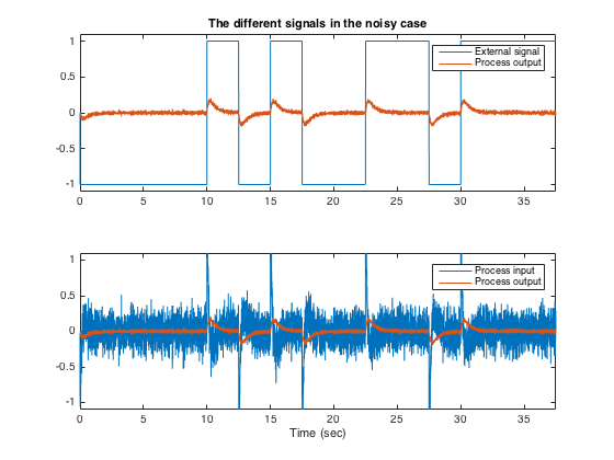
Let us have a look to the different noisy signals involved. Note in particular, the large level of noise on the process input
  subplot (2,1,1)
  plot(t,r,t,y),legend('External signal','Process output')
  axis([0 t(end) -1.1 1.1])
  title('The different signals in the noisy case')
  subplot (2,1,2)
  plot(t,u,t,y),legend('Process input','Process output')
  axis([0 t(end) -1.1 1.1])
  xlabel('Time (sec)')
Using this noisy output in the CLSRIVC routine with the previous input arguments:
Mclsrivc=clsrivc(data_yu,data_yr,[2 2 0],Mc)
Mclsrivc =
Continuous-time OE model:  y(t) = [B(s)/F(s)]u(t)
  B(s) = 0.9679 s + 0.9669

  F(s) = s^2 + 0.5478 s + 1.014

Parameterization:
   Polynomial orders:   nb=2   nf=2   nk=0
   Number of free coefficients: 4
   Use "polydata", "getpvec", "getcov" for parameters and their uncertainties.

Status:
Estimated using Contsid CLSRIVC method on time domain data.
Fit to estimation data: 70.51
FPE: 2.369e-04, MSE 2.367e-04
Let us again compare the identified model with the true process model. As seen below, they are still quite close
M0,
M0 =
Continuous-time OE model:  y(t) = [B(s)/F(s)]u(t) + e(t)
  B(s) = s + 1

  F(s) = s^2 + 0.5 s + 1

Parameterization:
   Polynomial orders:   nb=3   nf=2   nk=0
   Number of free coefficients: 5
   Use "polydata", "getpvec", "getcov" for parameters and their uncertainties.

Status:
Created by direct construction or transformation. Not estimated.
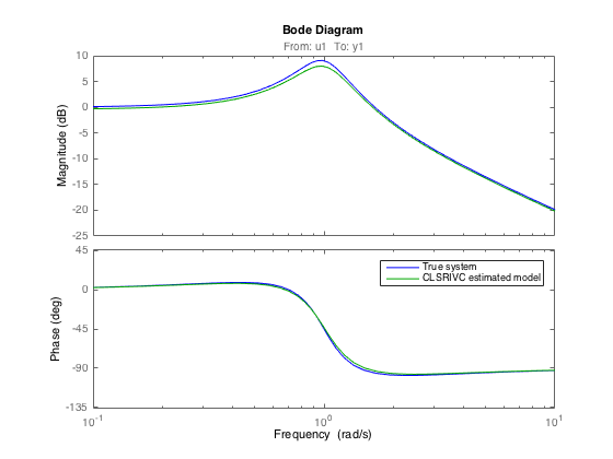
Let us compare the Bode diagrams of the true and the estimated model As you can see, the original and identified Bode diagrams are very close.
  close
  bode(M0,'b',Mclsrivc,'g')
  legend('True system','CLSRIVC estimated model')
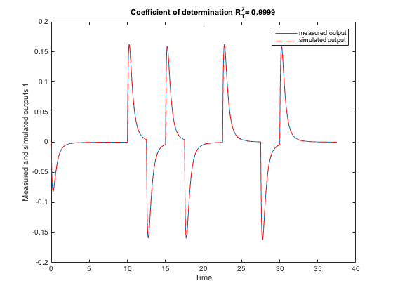
Let us now compare the model output with the measured output in the time-domain. Since we generated the data, we enjoy the luxury of comparing the model output to the noise-free system output. This can be done easily by using the COMPAREC routine which plots the measured and the simulated model outputs and displays the coefficient of determination RT2=1-var(y-ysim)/var(y). They coincide extremely well.
comparec(datadet_yu,Mclsrivc,1:N);
Additional Information
For more information on identification of continuous-time dynamic models visit the CONTSID Toolbox web page.