Estimating Continuous-time Transfer Function Models from Sampled Data
This example illustrates how you can use the CONTSID toolbox tools to determine a continuous-time model from sampled data by applying the general iterative system identification procedure. Learn how to generate some simulation data with the toolbox and then proceed systematically to estimate non-parametric and parametric models and also validate the identified model.
Contents
System Identification Procedure with the CONTSID
The identification procedure consists in designing an experiment (when possible) to collect input and output data and then in repeatedly selecting a model structure, computing the best model in the chosen structure, and evaluating the identified model. More precisely, the iterative procedure involves the following 5 steps: 1. Design an experiment and collect time-domain input/output data from the process to be identified. 2. Examine the data. Remove trends and outliers and select useful portions of the original data. 3. Define and select and a model structure (a set of candidate system descriptions) within which a model is to be estimated. 4. Estimate the parameters in the chosen model structure according to the input/output data and a given criterion of fit. 5. Examine the finally estimated model properties. If the model is good enough, then stop; otherwise go back to Step 3 and try another model set. Possibly also try other estimation methods (Step 4) or work further on the input/output data (Steps 1 and 2). As illustrated in this demo, the CONTSID toolbox includes tools for applying the general data-based modelling procedure.
The CONTSID toolbox may be seen as an add-on to the system identification toolbox for MATLAB. It uses the same data object, the same model object.
A simulation example: the Rao-Garnier benchmark
We consider a simulation example known as the Rao-Garnier benchmark. We first generate some data and illustrate how to use the different CONTSID toolbox routines to determine and validate a continuous-time model directly from the sampled data. The Rao-Garnier Benchmark is described as an COE model given by:
     y(t) = [B(s)/F(s)]u(t) + e(t)
where
       B(s)             -6400s + 1600
G(s) = ------ =  -------------------------------------
       F(s)      s^4 + 5s^3 + 408s^2 + 416s + 1600
where s denotes the differentiation operator. Create first an IDPOLY model structure object describing the continuous-time plant model. ...,'Ts',0) indicates that the system is time-continuous.
    B=[-6400 1600];
    F=[1 5 408 416 1600];
    M0=idpoly(1,B,1,1,F,'Ts',0);
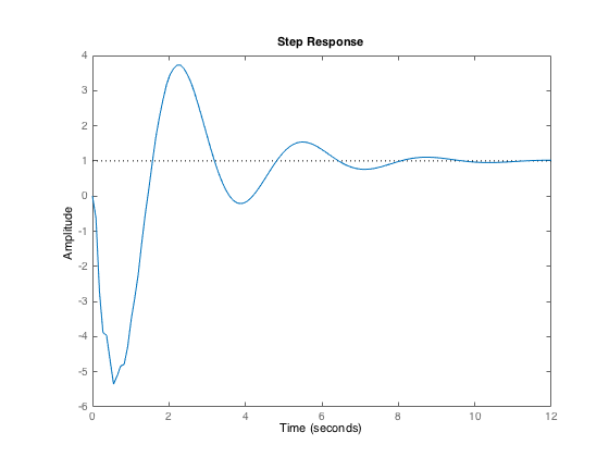
Plot the step response from which it can be observed that the system is non-minimum phase, with a zero in the right half plane.
    close all;
    step(M0);
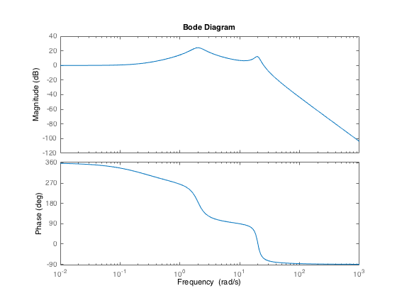
Plot now the frequency response from which, it can be seen that the system has two modes: one fast oscillatory mode around 20 rad/sec and one slow oscillatory mode around 2 rad/sec.
bode(M0);
Stage 1 - Experiment Design
The toolbox includes several functions to generate excitation signals: - SINERESP returns the exact steady-state response of a continuous-time model for a sum of sine signals. - PRBS generates a pseudo-random binary signal of maximum length. We choose here to send a PRBS of maximum length as input u. The sampling period Ts is chosen to be 0.01. A data object is first created that will be used to generate the simulated output. The input intersample behaviour is specified by setting the property 'Intersample' to 'zoh' since the input is piecewise constant here.
    u = prbs(10,7);
    N=length(u);
    Ts=0.01;
    datau = iddata([],u,Ts,'InterSample','zoh');
Simulating the system response to the PRBS excitation signal
The toolbox includes a routine SIMC to simulate the output signals given the model object. It is possible to specify the white noise level added the output by specifying the signal-to-noise ratio (SNR=10 dB here). The output of the SIMC function is the simulated noisy output stored in y. A data object is then created that includes both output and input data that will be given as input argument to the model structure determination and parameter estimation routines.
    snr=10;
    y = simc(M0,datau,snr);
    data = iddata(y,u,Ts,'InterSample','zoh');
Stage 2 - Data Analysis
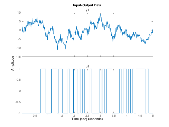
A first step in an identification application is to plot the data. Then it is recommended to remove the possible trend and faulty values (called outliers). The goal is to choose a part of the data that looks good and that is suitable for the model fit and validation. Let us have a look to a zoom part of the input and output signals. On basis of the time-domain data. The response to the PRBS is clearly observed except as long as the noise effect on the output.
    idplot(data,1:500);
    xlabel('Time (sec)')
Let us select the first 1000 data for the model identification.
data_est = data(1:1000);
Stage 3 - Model Structure Determination
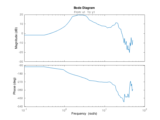
Selecting a model structure that is suitable to represent the system dynamics is probably the most difficult decision the practionner has to make. A good advice is to get some a priori information about the system order from a nonparametric model estimate. An estimate of the frequency response can be obtained for example by using the SPAFRD routine available in the System Identification toolbox. This routine estimates the frequency response by spectral analysis with frequency dependent resolution. The last input argument below specifies that the frequency response should be computed over 200 logarithmically spaced frequencies from 0.1 to 50 rad/sec. From the nonparametric estimate, it is obvious that at least two complex pole pairs and one or two complex zero pairs will be necessary.
    g=spafdr(data_est,[],{0.1,50,200});
    h=bodeplot(g);
Testing different model order structures
A natural way to find the most appropriate model orders is to compare the results obtained from model structures with different orders and delays. A model order selection function SRIVCSTRUC associated to the SRIVC model estimation algorithm allows the user to automatically search over a whole range of different model orders. Collect in a matrix NN all the model structure you want to investigate by specifying the miminal values [nb_min nf_min nk_min] and maximal values [nb_max nf_max nk_max] for the model structure. Then, a continuous-time model is fitted to the iddata object "data_est" for each of the structures in "NN". For each of these estimated models, different statistical measures are computed and used for the analysis.
    nb_min=1; nb_max=2;nf_min=3; nf_max=5;nk_min=0; nk_max=0;
    NN=[nb_min nf_min nk_min;
        nb_max nf_max nk_max];
    V=srivcstruc(data_est,[],NN);
Elapsed time : 0 h 0 min 19 s
Analyzing the different estimated model structures
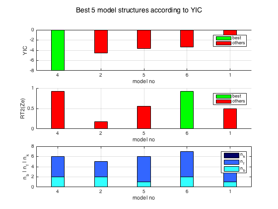
The different estimated model structures can be sorted according to one of the statistical measures (Young Information Criterion by default) are displayed with by using the SELCSTRUC function. From the table displayed, the best trade-off for both criteria YIC (the most negative) and associated RT2 (closer to 1) is here obtained for nn=[2 4 0] which is the true model order of the Rao-Garnier benchmark.
selcstruc(V);
 Tip for the choice of the model structure: Select the model
 that has the most negative YIC and highest associated RT2.


 The number of estimated models respecting the criteria of
 selection is equal to 6 over the 6 estimated.


 Table 1. Best 5 model structures according to YICs that respect
 the criteria (computation performed on estimation data set).
*****************************************************************


Table1 =

    no    np    nb    nf    nk      RT2        YIC      Niter     FPE        AIC         Cond        RT2v
    __    __    __    __    __    _______    _______    _____    ______    _______    __________    _______

    4     6     2     4     0     0.92021    -7.9756     5       1.1663    0.15381          4153    0.92021
    2     5     2     3     0     0.17475    -4.5717    10        13.07     2.5703        2115.2    0.17475
    5     6     1     5     0     0.55352    -3.6267    10        6.948     1.9385    1.3973e+06    0.55352
    6     7     2     5     0     0.92037    -3.3835     8        1.166     0.1536    6.8062e+08    0.92037
    1     4     1     3     0     0.49702    -1.1307    10       9.9386     2.2964        7493.6    0.49702


 Table 2. Best estimation performance indexes.
*****************************************************************


Table2 =

                 val      no
               _______    __

    RT2(Ze)    0.92037    6
    YIC        -7.9756    4
    Niter            5    4
    FPE          1.166    6
    AIC         0.1536    6
    RT2(Zv)    0.92037    6
Stage 4 - Parameter Estimation
We identify now a continuous-time model for this system from the noisy data object 'data_est' with the continuous-time model identification algorithm SRIVC. This routine implements the optimal instrumental variable method for continuous-time output error (COE) model. This estimator is reliable and it is recommended to use it as a first choice in practice. The extra information needed for the routine is the number of numerator and denominator parameters and number of samples for the delay of the model [nb nf nk] stored in the variable nn. The SRIVC identification algorithm can be used as follows:
    nn = [2 4 0];
    Msrivc = srivc(data_est,nn);
Diplaying the estimated model parameters
The estimated parameters together with their standard deviations can now be displayed as follows:
present(Msrivc)
Msrivc =
Continuous-time OE model:  y(t) = [B(s)/F(s)]u(t)
  B(s) = -6343 (+/- 122.5) s + 1710 (+/- 259.8)


  F(s) = s^4 + 4.727 (+/- 0.1763) s^3 + 407.4 (+/- 2.956) s^2 + 411.9 (
                                           +/- 10.86) s + 1605 (+/- 25.73)

Parameterization:
   Polynomial orders:   nb=2   nf=4   nk=0
   Number of free coefficients: 6
   Use "polydata", "getpvec", "getcov" for parameters and their uncertainties.

Status:
Estimated using Contsid SRIVC method on time domain data.
Fit to estimation data: 71.75
FPE: 1.166e+00, MSE 1.152e+00
More information in model's "Report" property.
Stage 5 - Model Validation
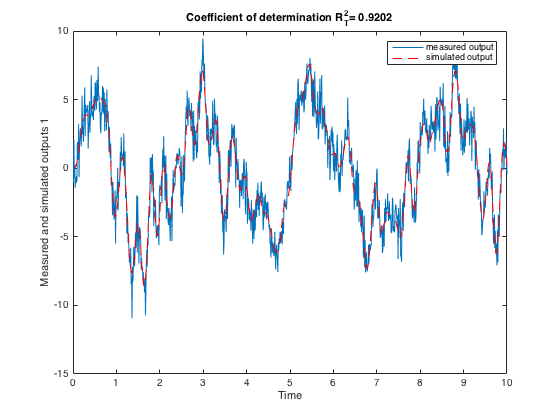
How good is this model? One way to find out is to simulate it and compare the model output with the measured output. We can use the COMPAREC routine to plot both outputs in an easy way. The fit is pretty good with a coefficient of determination very close to 1 which illustrates that the output variance is well explained by the model output.
    close
    comparec(data_est,Msrivc);
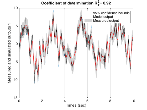
Plotting the confidence region
We can also use the COMPAREC routine in association with the SHADEDPLOT routine to plot the 95% confidence bounds. The plot confirms that both outputs coincide very well.
    [ys,esti]=comparec(data_est,Msrivc);
    t=(1:data_est.N)'*data_est.Ts;
    shadedplot(t,data_est.y,ys);
    xlabel('Times (sec)')
    title(['Coefficient of determination R_T^2= ',num2str(esti.RT2,3)])
    set(gca,'FontSize',14,'FontName','helvetica');
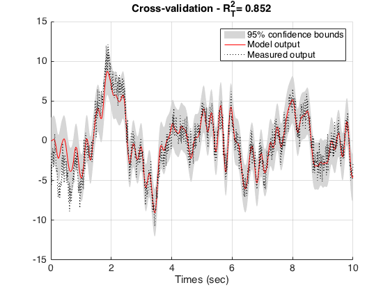
Cross-validation
It is a common practice to test the identified model on some data that were not used to fit the model. Let us select a part of the original data set that was not utilized to estimate the parameters.
We can again use the COMPAREC routine in association with the SHADEDPLOT routine to plot the 95% confidence bounds for the new dataset. The new plot shows that the estimated model can reproduce the system dynamics for a data that was not used for determining the parameters.
    data_val=data(3001:4000);
    [ys,esti]=comparec(data_val,Msrivc);
    t=(1:data_val.N)'*data_val.Ts;
    close
    shadedplot(t,data_val.y,ys);
    xlabel('Times (sec)')
    title(['Cross-validation - R_T^2= ',num2str(esti.RT2,3)])
    set(gca,'FontSize',14,'FontName','helvetica');
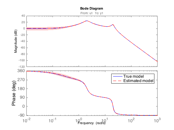
Validating the model in the frequency-domain
Let us eventually compare the Bode plots of the estimated model and the true system. The confidence regions corresponding to 3 standard deviations are also displayed. From the plot, they coincide very well with very small confidence regions.
    close
    bode(M0,'b-',Msrivc,'r--','sd',3,'fill')
    set(gca,'FontSize',14,'FontName','helvetica');
    legend('True model','Estimated model')
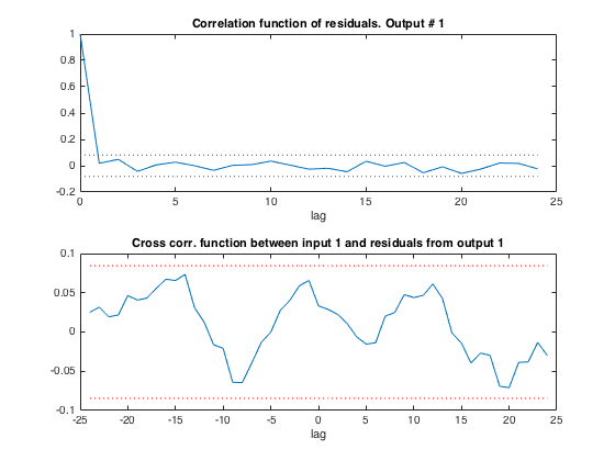
Residual analysis
We can also check the residuals (simulation error) of this model, and plot the autocorrelation of the residuals and the cross-correlation between the input and the residuals by using the RESIDC function We see that the residuals are white and totally uncorrelated with the input signal. We can thus be satisfied with the identified COE fourth-order model.
residc(data_est,Msrivc);
Additional Information
For more information on identification of continuous-time dynamic models visit the CONTSID Toolbox web page.